Evolutionary Algorithm Problem 111

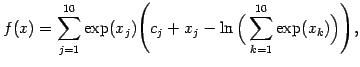
This is another test example to see if the CE algorithm produces more desirable results. The minimization problem taken from [4], problem 111 on pg 120, is similar to Problem 112 above except we are dealing with $\exp(\mathbf{x}$ ) now. The objective function is:

$$f(x)= \sum_{j=1}^{10} \exp(x_j) \Bigg(c_j + x_j - \ln\Big(\sum_{k=1}^{10} \exp(x_k)\Big)\Bigg),$$

subject to the constraints:

$\exp(x_1) + 2\exp(x_2) + 2\exp(x_3) + \exp(x_6) + \exp(x_{10}) - 2 = 0$

$\exp(x_4) + 2\exp(x_5) + \exp(x_6) + \exp(x_7) -1 = 0$

$\exp(x_3) + \exp(x_7) + \exp(x_8) + 2\exp(x_9) + \exp(x_{10}) = 0$

$-100 \le x_i \le 100 (i=1, \ldots, 10)$ ,

where

$c_1=-6.089; c_2=-17.164; c_3=-34.054; c_4=-5.914; c_5=-24.721;$

$c_6=-14.986; c_7=-24.100; c_8=-10.708; c_9=-26.662; c_{10}=-22.179.$

The previous best known solution in [4] was

$\mathbf{x}^{*} = (-3.201212, -1.912060, -0.2444413, -6.537489, -0.7231524,$

             $-7.267738, -3.596711, -4.017769, -3.287462, -2.335582)$ ,

and $f(\mathbf{x}^{*}) = -47.76109026$ .

The optimal solution found by the CE algorithm was

$\mathbf{x}^{*} = (-3.20239422280305, -1.91211352220761, 0.244404027043058,$

         $-6.56117799901427, -0.723117923945733, -7.26779073659076,$

         $-3.59669401608479, -4.01983995665254, -3.28743607295152,$

         $-2.33552331245161)$ ,

and $f(\mathbf{x}^{*}) = -47.7610907529719$ . As the initial mean and initial standard deviation in the CE algorithm were derived from the previous best known solution, every iteration produces results that were better than the above solution.

gen.m - generation of samples, satifying constraints.

normt1.m - generates truncated normals

opt.m - main program

S.m - objective function