Stategies to Increase Accuracy

1. Injection. The idea behind the injection modification, first proposed in [2], is to inject extra variance into the sampling distribution in order to avoid premature ``shrinkage'' of the distribution. More precisely, let Sstar denote the best performance found at some iteration t, and sigstar the largest standard deviation at that iteration. If sigstar is sufficiently small, and Ssdiff = |Sstar(t) - Sstar(t-1)| is also small, then add a constant times Ssdiff to each standard deviation, for some fixed constant, say 1 - 100.

2. Increasing $N$ , decreasing $\varrho$ . This is a basic idea to increase the accuracy. One simply increases the sample size, while, possibly, decreasing the rarity parameter. Alternatively, the sample size is increased while the elite sample size is kept constant. A more sophisticated approach is given by the FACE algorithm.
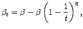
3. Modified or dynamic smoothing. When the smoothing parameter alpha is large, say 0.9, the convergence to a degenerate distribution may happen too quickly, which would ``freeze'' the algorithm in a sub-optimal solution. One way to prevent this from happening is to use dynamic smoothing [6] where at iteration t the variance of the normal sampling distribution is updated using a smoothing parameter
   $$\beta_t = \beta - \beta \left(1 - \frac{1}{t}\right)^q,$$
   where q is a small integer (typically between 5 and 10) and beta is a large smoothing constant (typically between 0.8 and 0.99). The mean parameter can be updated in the conventional way, with constant smoothing parameter. By using a time dependent smoothing parameter the speed of convergence to the degenerate case is polynomial instead of exponential. A difficulty with dynamic smoothing is that when the optimal function value is unknown it is difficult to formulate a good stopping criterion due to the slower convergence of the algorithm

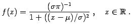
4. Heavy-tailed sampling. Instead of the usual normal sampling distribution, one could use a distribution with a heavier tail, such as the Cachy distribution with location parameter mu and scale parameter sigma. That is, with pdf
   $$f(x) = \frac{(\sigma \pi)^{-1}}{1 + ((x - \mu)/\sigma)^2}\;, \quad x \in \mathbb{R}\;.$$
   The advantages are that (1) injection or dynamic smoothing may not be necessary, (2) generation from a Cauchy distribution and also a truncated Cauchy distribution is easy. A disadvantage is that the maximum likelihood estimators for mu and sigma are not easily derived. However, the median of the data and the range (maximum - minumum) are accurate estimators of the location and scale parameters, respectively.